Setting Up a Spreadsheet for Recipe Conversions
Setting Up a Spreadsheet for Recipe Conversions
This resource is intended to walk users through the process of setting up a spreadsheet to help convert volumetric recipes to weight-based formulas. This exercise will use a predetermined recipe to show how this process is done, but the spreadsheet made can be easily adapted for your own product. For more information on the importance of measuring ingredients using weight, please refer to our Scale Technique and Recipe Consistency and Recipe Formulation videos.
- Either open up Microsoft Excel (if you have the program), or go to Google Sheets and setup a free google account if you don’t already have one (the screenshots for this are from google sheets). Both programs function in similar ways, so you will be able to follow these instructions for either program.
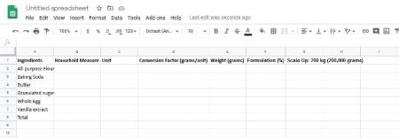
- Starting in square A1, enter ingredients, household measure, unit, conversion factor (grams/unit), weight (grams), formulation %, and scale up: 200 kg (200,000 grams), moving left to right. Starting in square A2, enter all-purpose flour, baking soda, butter, granulated sugar, whole egg, vanilla extract, and total, moving top to bottom. Your spreadsheet should resemble the image below:

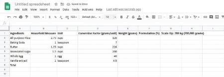
- Starting in square B2 enter the following numbers, top to bottom: 2.75, 1, 1.25, 1.5, 1, and 1. Starting with square C2, enter the following words, top to bottom: cups, teaspoon, cups, cups, egg, teaspoon. Lastly, starting in square D2, enter the following numbers, top to bottom: 120, 7, 226, 200, 40, 4.5. Your spreadsheet should resemble the image below:

- In square E2 enter the following formula “=(B2*D2)” (do not include the “”) then hit enter. The square should read “330”. This formula is used to convert the cup measure to weight in grams, by multiplying the household measure for flour (2.75 cups) and the conversion factor (of 120 grams per cup), to reach 330 grams of flour in the batch.
- Hover your mouse over the bottom right corner of the E2 square. Your mouse should turn into a + icon. Click, and drag the mouse down to the bottom of row 7. The equation will fill in the blanks for the rest of the conversions for the other ingredients. Your table should now look like the second image below.

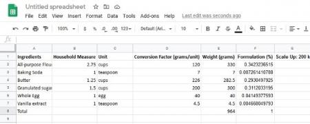
- In square E8, enter the following formula “=SUM(E2:E7)” (don’t include the “”), and hit enter. This will give you the total weight of the batch, which should read 964.
- It’s now time to convert the weight formula to formula %. In square F2, enter the following formula “=(E2/$E$8)” (don’t include the “”), and hit enter (note: the $ are a formula indicator that locks the value of the square when scrolling/dragging the formula to other squares). The square should read 0.3423… This means that the batch is 34.23% flour, by weight. Click in the bottom right corner of square F2, and drag down through row 7, just as you did in step 5 to fill in the rest of the ingredient formula %’s. If you drag through row 8, you should see a “1” in row 8, indicating that you entered the formula correctly. Your spreadsheet should now look like the image below.

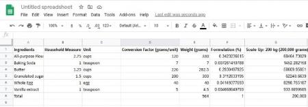
- The last step is to scale up the formula. In square G2, enter the following formula:
“=(F2*200000)” (don’t include the “”), and hit enter. The square should now read 68464.73… This means for a 200,000g batch, there are 68,464.73 grams of flour. Click the bottom right corner and drag down through row 8, just as you did in steps 5 and 7. The new ingredient weights for a 200,000 gram batch will now show. That’s all! Your converted formula is complete.
